注釈
Go to the end をクリックすると完全なサンプルコードをダウンロードできます.
球体メッシュを複数の方法で作成する#
この例では、さまざまな方法でメッシュを作成する方法を示しています。
from __future__ import annotations

import numpy as np

import pyvista as pv
シンプルな球体#
球メッシュを取得する最も簡単な方法は pyvista.Sphere() を使うことです。
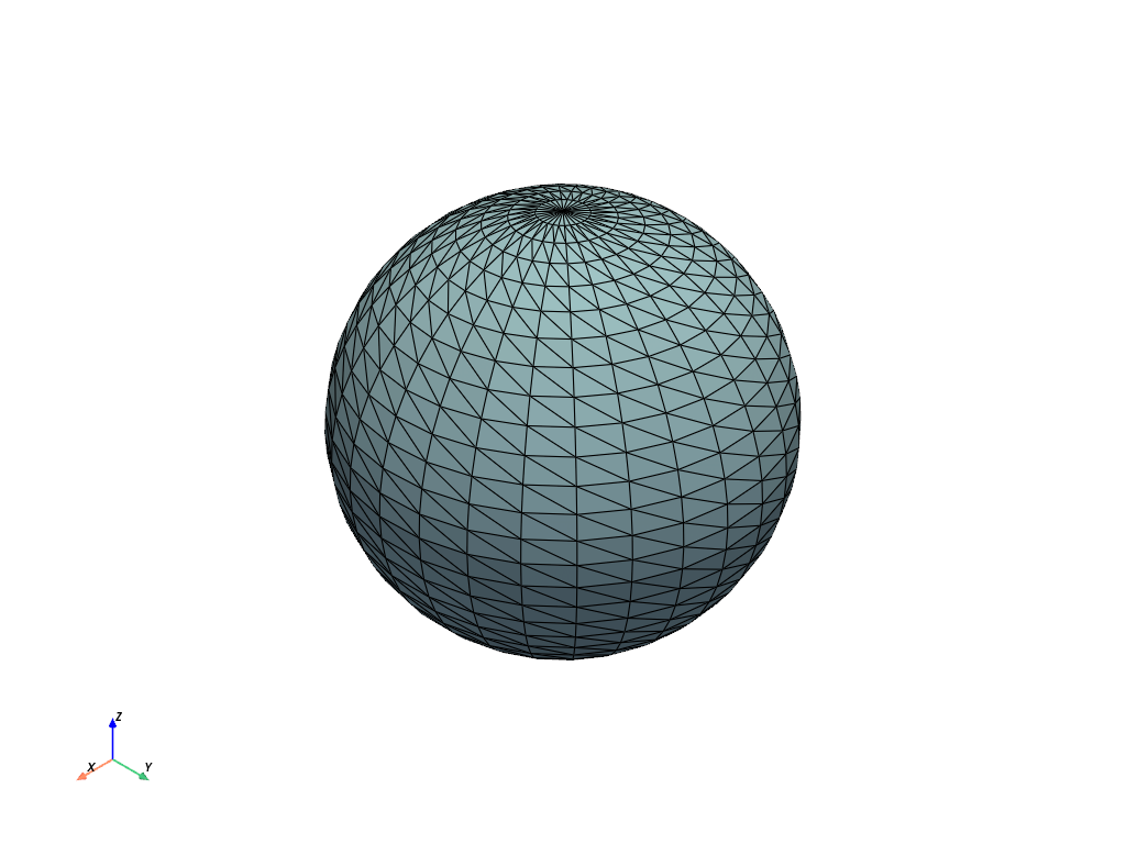
これで pyvista.PolyData メッシュ、つまり2Dサーフェスが得られます。
この場合、 manifold となり、ボリュームを囲みます。 これを示すために、点/セルが抽出されないことからわかるように、メッシュには境界がありません。
boundaries = mesh.extract_feature_edges(
    non_manifold_edges=True, feature_edges=False, manifold_edges=False
)
boundaries
セルは TRIANGLE のセルです。 例えば、最初のセルは
mesh.get_cell(0).type
<CellType.TRIANGLE: 5>
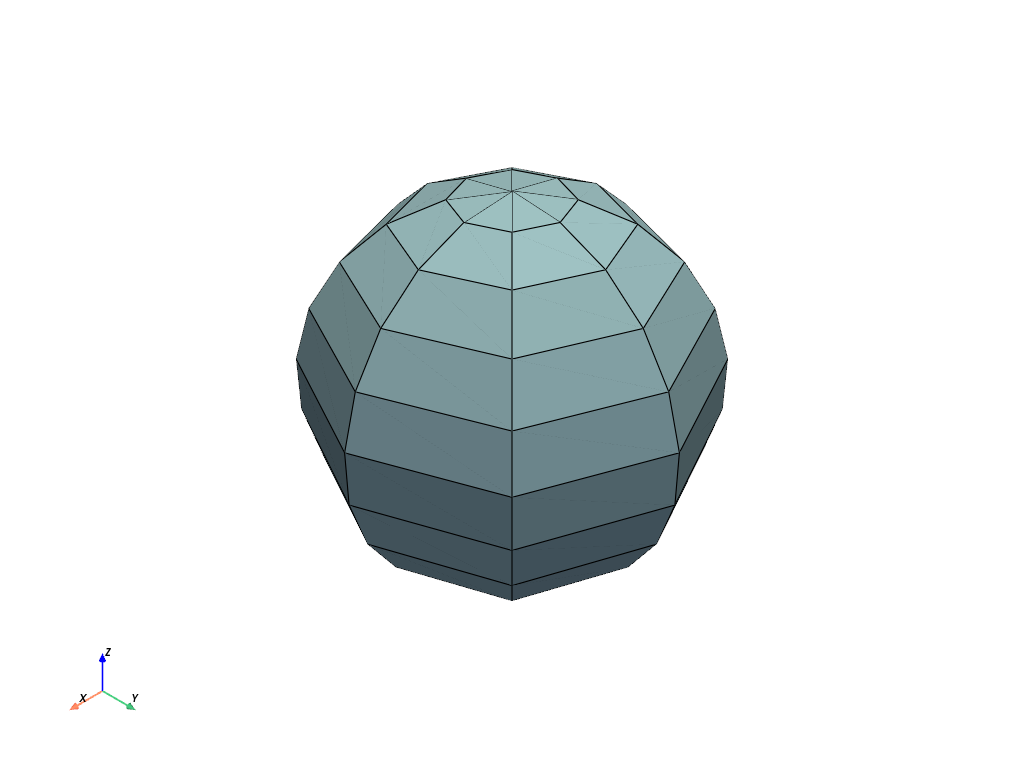
球の構造化四辺形メッシュ#
メッシュの構造は重要である。 三角形のメッシュの代わりに、i-j-kの順序を持つ構造化メッシュがあると便利です。 これによってセルの接続を単純化することができます。
pyvista.spherical_to_cartesian() を使用して、球座標の規則的なグリッドとして点を生成します。 ここでは、 theta は方位角であり、地球上の経度に似ているという慣例を使用します。 phi は極角で、地球上の緯度に似ています。
The mesh has QUAD cells. The cells that look triangular
at the poles are actually degenerate quadrilaterals, i.e. two
points are coincident at the pole, as will be shown later.
mesh.plot(show_edges=True)
メッシュの型は pyvista.StructuredGrid です。
最初のセルは一番上の極にあり、 QUAD セルです。
cell = mesh.get_cell(0)
cell.type
<CellType.QUAD: 9>
最初のセルには2つの縮退点があります。
array([[0.        , 0.        , 0.5       ],
       [0.14086628, 0.        , 0.47974649],
       [0.0996075 , 0.0996075 , 0.47974649],
       [0.        , 0.        , 0.5       ]])
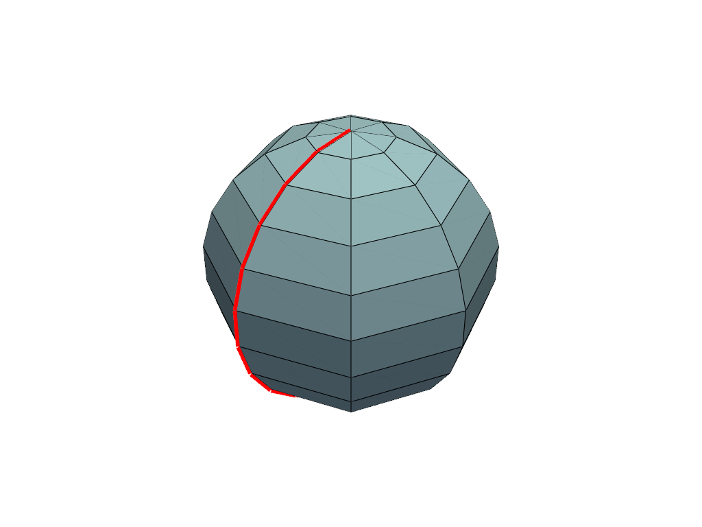
方位角成分の始点と終点に沿った '継ぎ目' の両側のセルはつながっていません。 これらは境界エッジを抽出することで検出できます。
boundaries = mesh.extract_feature_edges(
    non_manifold_edges=True, feature_edges=False, manifold_edges=False
)
boundaries
メッシュの境界エッジをプロットすることで、これを視覚化します。
pl = pv.Plotter()
pl.add_mesh(mesh, show_edges=True)
pl.add_mesh(boundaries, line_width=10, color='red')
pl.show()
球の四辺形メッシュの生成#
この例では、より複雑なメッシュを定義する方法を示しています。
In contrast to the example above, this example generates a mesh
that does not have degenerate points at the poles. TRIANGLE cells
will be used at the poles. First, regenerate the structured data.
We do not want duplicate points, so remove the duplicate in theta, which
results in 8 unique points in theta. Similarly, the poles at phi=0 and
phi=pi will be handled separately to avoid duplicate points, which
results in 10 unique points in phi. Remove these from the grid in spherical
coordinates.
Use pyvista.spherical_to_cartesian() to generate cartesian coordinates for points in the (N, 3)
format required by PyVista. Note that this method results in
the theta variable changing the fastest.
最初と最後の点が極点です。
First we will generate the cell-point connectivity similar to the
previous examples. At the poles, we will form triangles with the pole
and two adjacent points from the closest ring of points at a given phi
position. Otherwise, we will form quadrilaterals between two adjacent points
on consecutive phi positions.
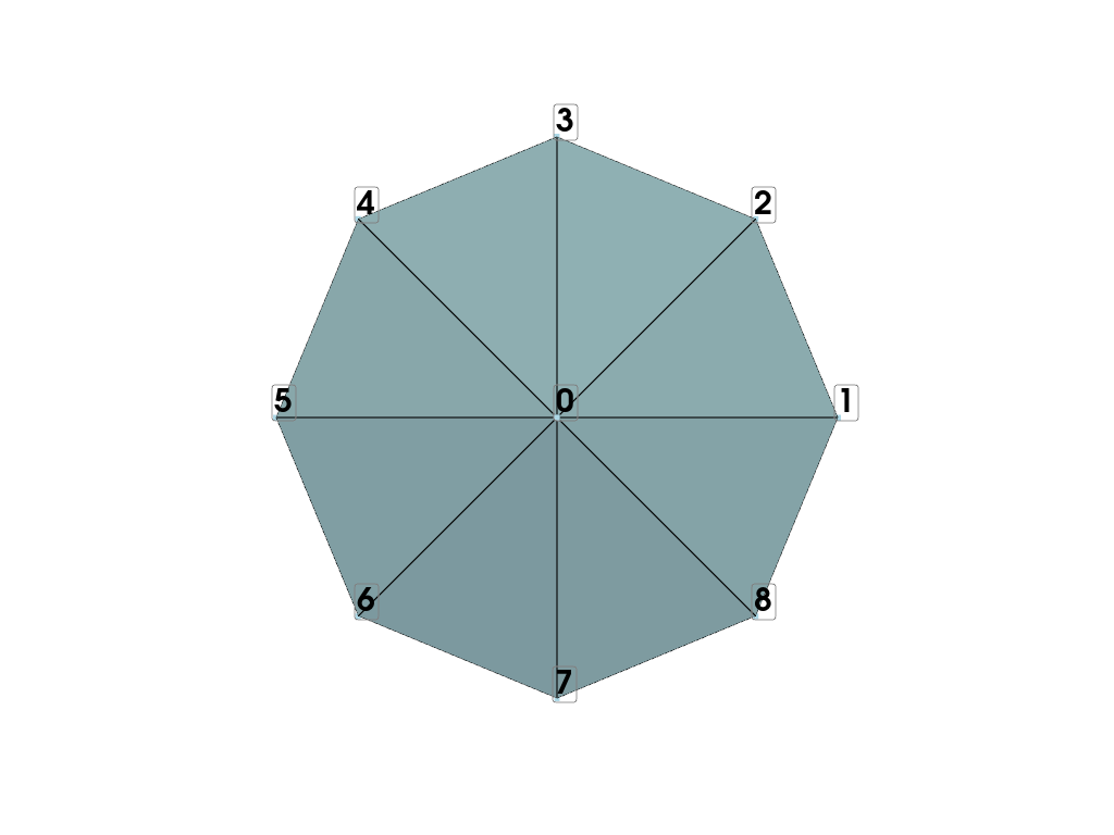
The first triangle in the mesh is point id 0, i.e. the pole, and
the first two points at the first phi position, id's 1 and 2.
the next triangle contains the pole again and the next set of points,
id's 2 and 3 and so on. The last point in the ring, id 8 connects
to the first point in the ring, 1, to form the last triangle. Exclude it
from the loop and add separately.
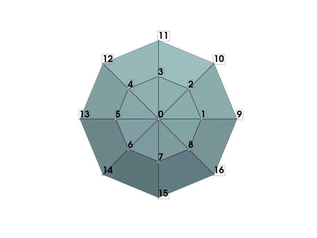
これまでのメッシュの接続性を示します。
points_to_label = tuple(range(ntheta + 1))
mesh = pv.PolyData(points, faces=faces)
pl = pv.Plotter()
pl.add_mesh(mesh, show_edges=True)
pl.add_point_labels(
mesh.points[points_to_label, :], points_to_label, font_size=30, fill_shape=False
)
pl.view_xy()
pl.show()
Next form the quadrilaterals. This process is the same except
by connecting points across two levels of phi. For point 1
and point 2, these are connected to point 9 and point 10. Note
for quadrilaterals it must be defined in a consistent direction.
Again, the last point(s) in the theta direction connect back to the
first point(s).
最初の4分の1レイヤーでメッシュの接続性を示します。
points_to_label = tuple(range(ntheta * 2 + 1))
mesh = pv.PolyData(points, faces=faces)
pl = pv.Plotter()
pl.add_mesh(mesh, show_edges=True)
pl.add_point_labels(
mesh.points[points_to_label, :],
points_to_label,
font_size=30,
fill_shape=False,
always_visible=True,
)
pl.view_xy()
pl.show()
Next we loop over all adjacent levels of phi to form all the quadrilaterals and add the layer of triangles on the ending pole. Since we already formed the first layer of quadrilaterals, let's start over to make cleaner code.
faces = []
for i in range(1, ntheta):
    faces.extend([3, 0, i, i + 1])

faces.extend([3, 0, ntheta, 1])
for j in range(nphi - 1):
for i in range(1, ntheta):
faces.extend(
[4, j * ntheta + i, j * ntheta + i + 1, i + (j + 1) * ntheta + 1, i + (j + 1) * ntheta]
)
faces.extend([4, (j + 1) * ntheta, j * ntheta + 1, (j + 1) * ntheta + 1, (j + 2) * ntheta])
for i in range(1, ntheta):
faces.extend([3, nphi * ntheta + 1, (nphi - 1) * ntheta + i, (nphi - 1) * ntheta + i + 1])
faces.extend([3, nphi * ntheta + 1, nphi * ntheta, (nphi - 1) * ntheta + 1])
ここでは pyvista.PolyData メッシュを使いますが、 pyvista.UnstructuredGrid を使うこともできます。
mesh = pv.PolyData(points, faces=faces)
This mesh is manifold like pyvista.Sphere().
To demonstrate this, there are no boundaries on the mesh
as indicated by no points/cells being extracted.
boundaries = mesh.extract_feature_edges(
    non_manifold_edges=True, feature_edges=False, manifold_edges=False
)
boundaries
すべてのポイントラベルは、プロットされたときに乱雑になるので、最終的なプロットに加えないでください。
mesh.plot(show_edges=True)

Total running time of the script: (0 minutes 1.350 seconds)