ボリュームレンダリング

pyvista.ImageData または3 D NumPy配列のようなボリュームレンダリングの均一メッシュタイプ．

これはまた pyvista.ImageData.extract_subset() フィルタを使用して pyvista.ImageData から関心領域 (VOI) を抽出する方法を探求します．

from __future__ import annotations

import numpy as np

import pyvista as pv
from pyvista import examples


# Download a volumetric dataset
vol = examples.download_knee_full()
vol

Header	Data Arrays
ImageData Information N Cells 10225800 N Points 10368384 X Bounds 0.000e+00, 1.497e+02 Y Bounds 0.000e+00, 1.786e+02 Z Bounds 0.000e+00, 2.000e+02 Dimensions 208, 248, 201 Spacing 7.230e-01, 7.230e-01, 1.000e+00 N Arrays 1	Name Field Type N Comp Min Max SLCImage Points uint8 1 0.000e+00 1.740e+02

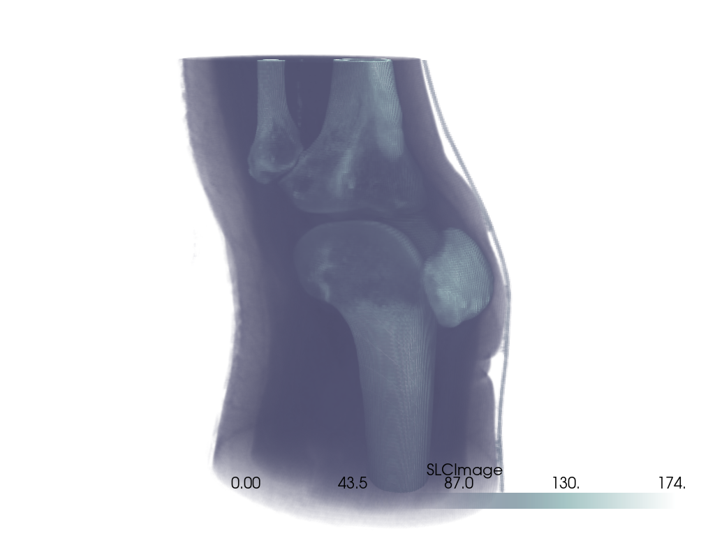
シンプルボリュームレンダー

# A nice camera position
cpos = [(-381.74, -46.02, 216.54), (74.8305, 89.2905, 100.0), (0.23, 0.072, 0.97)]

vol.plot(volume=True, cmap='bone', cpos=cpos)

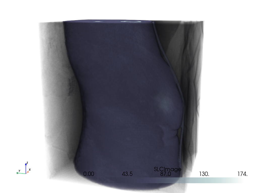
不透明度マッピング

または，以下のように pyvista.Plotter.add_volume() メソッドを使用します．ここでは，シグモイドへのデフォルト以外の不透明度マッピングを使用することに注意してください．

pl = pv.Plotter()
pl.add_volume(vol, cmap='bone', opacity='sigmoid')
pl.camera_position = cpos
pl.show()

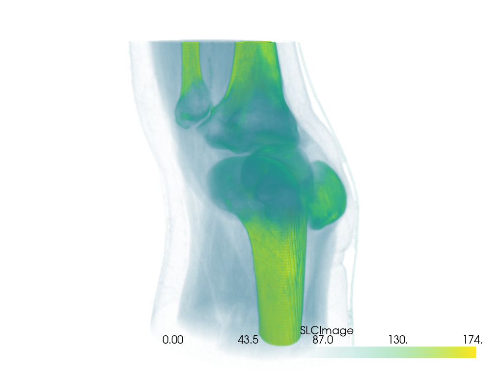
カスタム不透明度マッピングを使用することもできます．

opacity = [0, 0, 0, 0.1, 0.3, 0.6, 1]

pl = pv.Plotter()
pl.add_volume(vol, cmap='viridis', opacity=opacity)
pl.camera_position = cpos
pl.show()

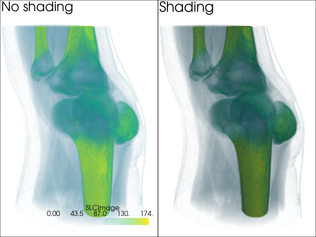
shade オプションを使用してボリュームレンダリングを行う場合は，シェーディングテクニックを使用することもできます．

pl = pv.Plotter(shape=(1, 2))
pl.add_volume(vol, cmap='viridis', opacity=opacity, shade=False)
pl.add_text('No shading')
pl.camera_position = cpos
pl.subplot(0, 1)
pl.add_volume(vol, cmap='viridis', opacity=opacity, shade=True)
pl.add_text('Shading')
pl.link_views()
pl.show()

かっこいいボリュームの例

ここでは，クールなボリュームレンダリングの例をいくつか紹介します．

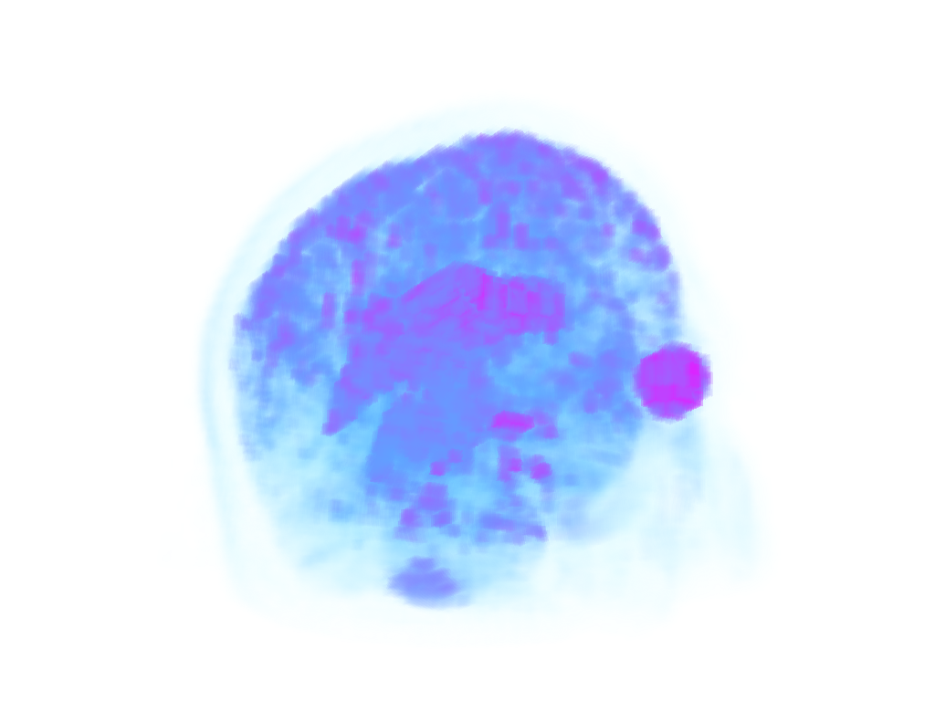
ヘッドデータセット

head = examples.download_head()

pl = pv.Plotter()
pl.add_volume(head, cmap='cool', opacity='sigmoid_6', show_scalar_bar=False)
pl.camera_position = [(-228.0, -418.0, -158.0), (94.0, 122.0, 82.0), (-0.2, -0.3, 0.9)]
pl.camera.zoom(1.5)
pl.show()

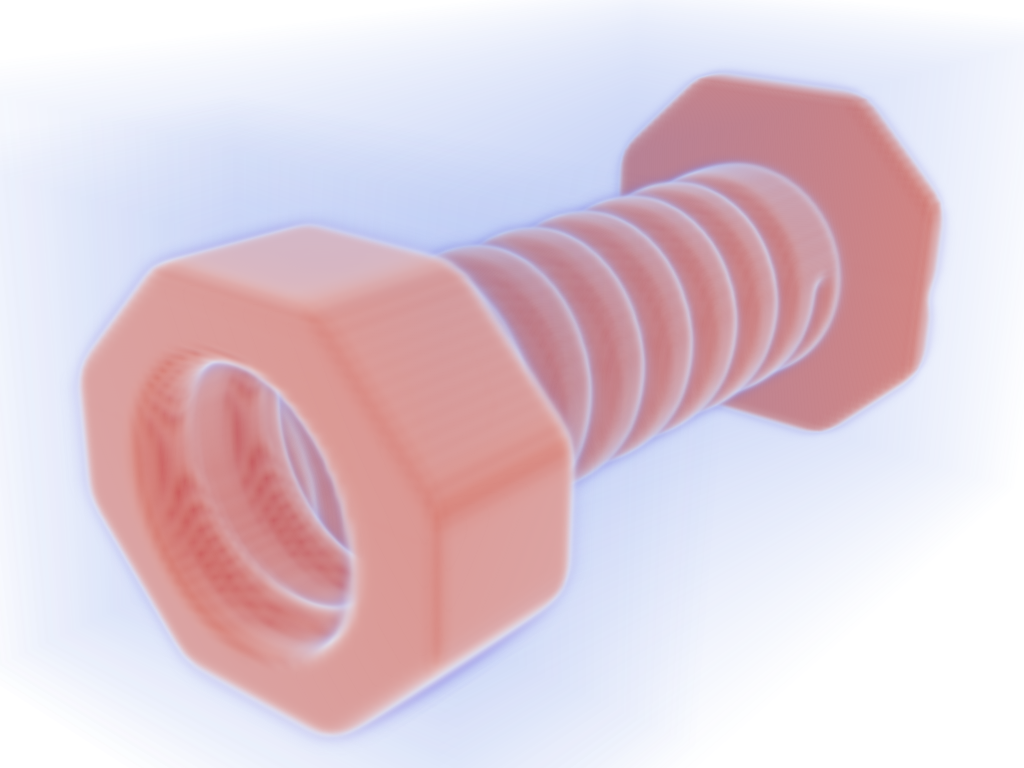
ボルト・ナット式マルチブロックデータセット

注釈

ここでは，より魅力的なプロットを作成するために，個々のセルのスカラーを滑らかにするために，補間を 'linear' に設定したことを確認してください． bolt_nut は pyvista.MultiBlock というデータセットなので， add_volume が返すアクターは 2 つになります．

bolt_nut = examples.download_bolt_nut()

pl = pv.Plotter()
actors = pl.add_volume(bolt_nut, cmap='coolwarm', opacity='sigmoid_5', show_scalar_bar=False)
actors[0].prop.interpolation_type = 'linear'
actors[1].prop.interpolation_type = 'linear'
pl.camera_position = [(127.4, -68.3, 88.2), (30.3, 54.3, 26.0), (-0.25, 0.28, 0.93)]
cpos = pl.show(return_cpos=True)

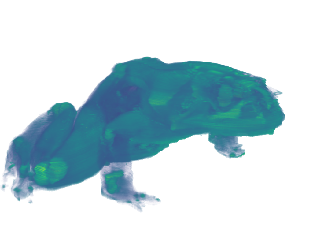
カエルデータセット

frog = examples.download_frog()

pl = pv.Plotter()
pl.add_volume(frog, cmap='viridis', opacity='sigmoid_6', show_scalar_bar=False)
pl.camera_position = [(929.0, 1067.0, -278.9), (249.5, 234.5, 101.25), (-0.2048, -0.2632, -0.9427)]
pl.camera.zoom(1.5)
pl.show()

VOIの抽出

pyvista.ImageDataFilters.extract_subset() フィルタを使用して，ボリュームレンダリングの対象となるボリューム/サブセットボリュームを抽出します．これは，特に大きなボリュームを処理し，特定の領域のみをボリュームレンダーする場合に理想的です．

# Load a particularly large volume
large_vol = examples.download_damavand_volcano()
large_vol

Header	Data Arrays
ImageData Information N Cells 11003760 N Points 11156040 X Bounds 4.130e+05, 6.920e+05 Y Bounds 3.864e+06, 4.096e+06 Z Bounds -5.479e+04, 5.302e+03 Dimensions 280, 233, 171 Spacing 1.000e+03, 1.000e+03, 3.535e+02 N Arrays 1	Name Field Type N Comp Min Max data Points float32 1 9.782e-15 1.000e+02

opacity = [0, 0.75, 0, 0.75, 1.0]
clim = [0, 100]

pl = pv.Plotter()
pl.add_volume(
    large_vol,
    cmap='magma',
    clim=clim,
    opacity=opacity,
    opacity_unit_distance=6000,
)
pl.show()

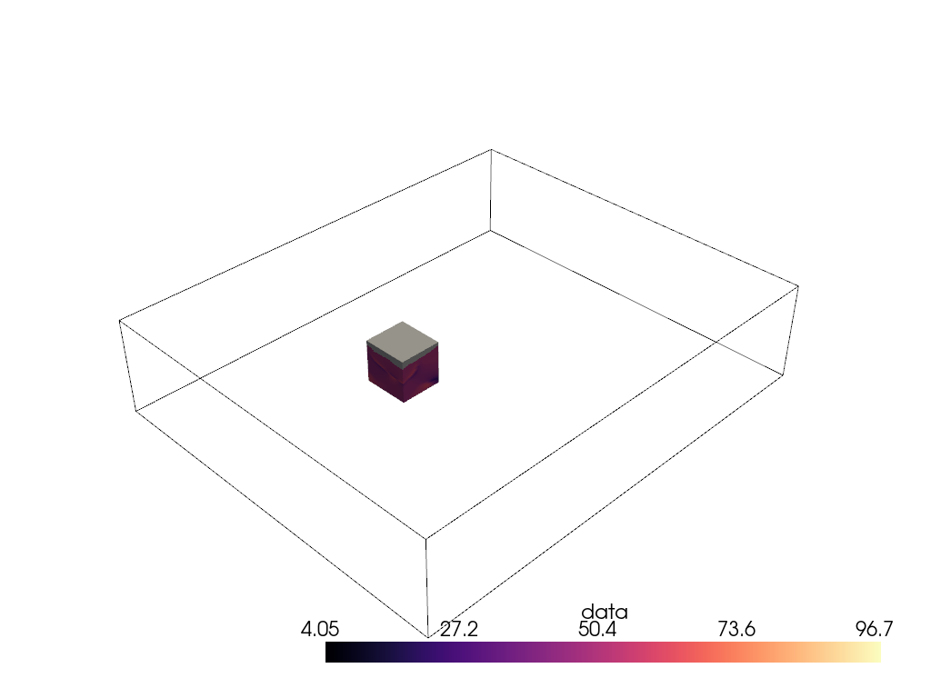
わあ，すごいボリュームだ．全体をボリュームレンダリングしたくはないでしょう．火山の下の興味深い地域を抽出してみましょう．

抽出する領域は，x軸上の節点175と200の間，y軸上の節点105と132の間，およびz軸上の節点98と170の間になります．

voi = large_vol.extract_subset([175, 200, 105, 132, 98, 170])

pl = pv.Plotter()
pl.add_mesh(large_vol.outline(), color='k')
pl.add_mesh(voi, cmap='magma')
pl.show()

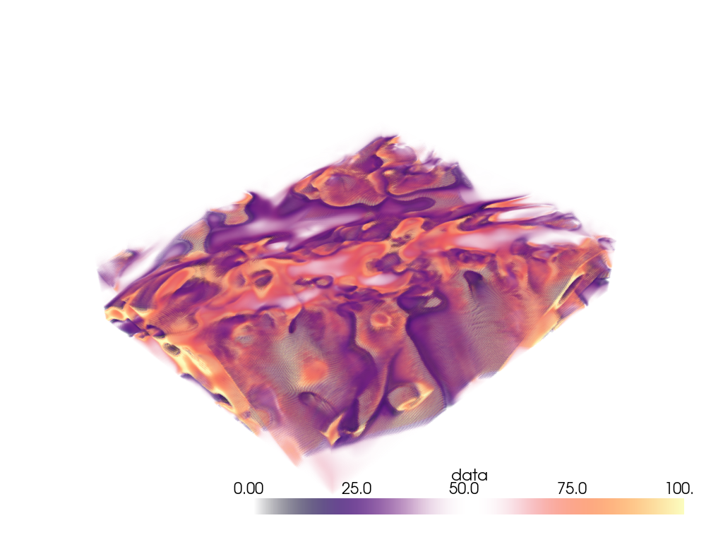
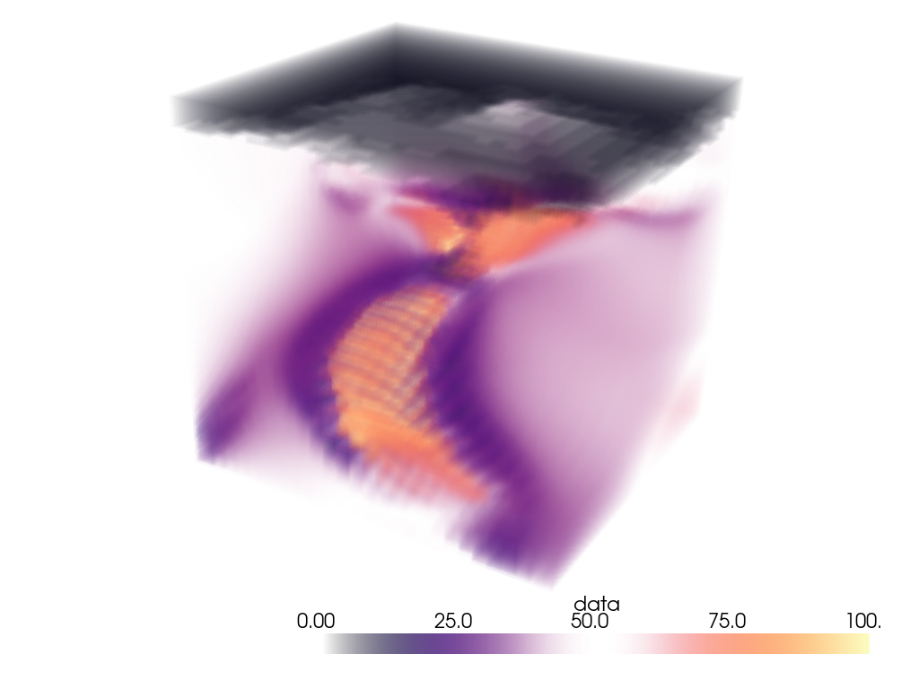
ああ，だいぶよくなりました．次に，その対象領域をボリュームレンダリングします．

pl = pv.Plotter()
pl.add_volume(voi, cmap='magma', clim=clim, opacity=opacity, opacity_unit_distance=2000)
pl.camera_position = [
    (531554.5542909054, 3944331.800171338, 26563.04809259223),
    (599088.1433822059, 3982089.287834022, -11965.14728669936),
    (0.3738545892415734, 0.244312810377319, 0.8947312427698892),
]
pl.show()

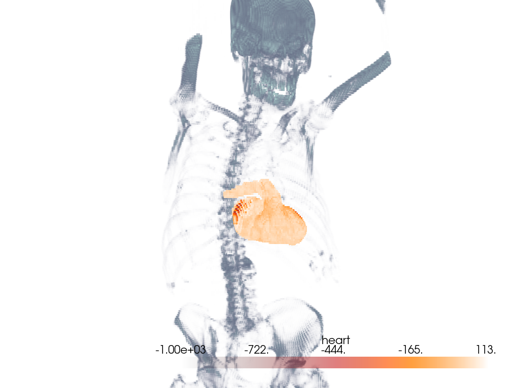
セグメンテーションマスク付きボリューム

Visualize a medical image with a corresponding binary segmentation mask.

For this example, we use download_whole_body_ct_male() though download_whole_body_ct_female(), or any other dataset with a corresponding label or mask may be used.

Load the dataset and get the ct image and a mask image. Here, a mask of the heart is used.

dataset = examples.download_whole_body_ct_male()
ct_image = dataset['ct']
heart_mask = dataset['segmentations']['heart']

Use the segmentation mask to isolate the heart in the CT image.

Initialize a new array and image with CT background values. Here, we set the scalar values to -1000 which typically corresponds to air (low density).

heart_array = np.full_like(ct_image.active_scalars, -1000)

Extract the intensities for the heart segment. We use heart mask's array to mask the CT image to only extract the intensities of interest.

ct_image_array = ct_image.active_scalars
heart_mask_array = heart_mask.active_scalars
heart_array[heart_mask_array == True] = ct_image_array[heart_mask_array == True]  # noqa: E712

Add the masked array to the CT image as a new set of scalar values.

ct_image['heart'] = heart_array

プロットを作成します．

For the CT image, the opacity is set to a sigmoid function to show the subject's skeleton. Since different images have different intensity distributions, you may need to experiment with different sigmoid functions. See add_volume() for details.

pl = pv.Plotter()

# Add the CT image.
pl.add_volume(
    ct_image,
    scalars='NIFTI',
    cmap='bone',
    opacity='sigmoid_15',
    show_scalar_bar=False,
)

# Add masked CT image of the heart and use a contrasting color map.
_ = pl.add_volume(
    ct_image,
    scalars='heart',
    cmap='gist_heat',
    opacity='linear',
    opacity_unit_distance=np.mean(ct_image.spacing),
)

# Orient the camera to provide a latero-anterior view.
pl.view_yz()
pl.camera.azimuth = 70
pl.camera.up = (0, 0, 1)
pl.camera.zoom(1.5)
pl.show()

Tags: medical plot